Building Dashboards in Excel > Part 2 - Tables
When you create dashboards with Excel, well organized and structured data is the key to succes! This article is about Excel Tables, what you have to know about working with tables and what options Excel offer to work with structured data.
1) EXCEL AND TABLES
A table is an important but underestimated feature in Excel. A table is a range with structured data. It makes managing and analyzing a group of related data easier.
In a table, a row can contain information about customers where a column contains more specific information about all of the customers.
In Excel, you can recognize a table in a couple of ways. First of all, you will find a Design tab on the ribbon when a table is active. You can also recognize a table from a little blue marker at the bottom right cell of your data.
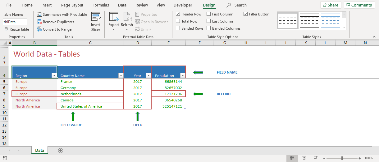
1.1) Tables - Properties
A table is actually no more than a worksheet range with the following properties:
-
- Table Range – A worksheet range with records
- Record – A collection of fields
- Field – A single type of information about a record
- Field Name – A unique name assigned to every field
- Field Value – The value in a field
Tables are easy to create, but do require some rules for the best results:
-
- Use only one row (the top row) for the Field Names
- Field Names MUST be unique and MUST be text
- Some Excel commands identify the size of a Table. To not “confuse” Excel, try to use only one table on a worksheet. When you have more than one table, use a separate worksheet for each table!
- Don’t type non-table data directly next to a table. Excel might misinterpret the table range!
!! A table can filter records. This means that some rows might not be visible after a filter command. Therefore, you should never place data that does not belong to a table to the left or to the right of that table!
!! When you don’t know if you are working with a range or a table, check the bottom right corner of your dataset. If you see a little blue marker, you are working with a table!
1.2) Tables - Creating a table
A range of cells can be converted into a table. This has some nice advantages, as a table offers lots of extra functionalities. You can convert a range of cells into a table with three mouse clicks.
-
- Select a cell inside the range of cells that you want to convert into a table
- Click the Insert tab from the ribbon
- Click Table
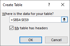
When you structured your data according to the principles of proper database design, Excel recognizes the range for a possible table and displays the Create Table dialog, shown in Figure 1‑2. Click OK to convert the selected range into a table.
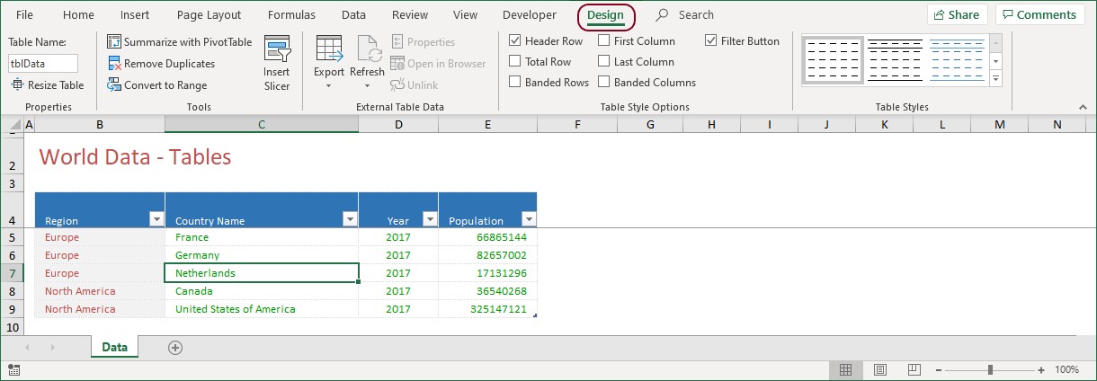
Figure 1‑3 shows the selected table on the worksheet. Because the table is active, the ribbon shows the Design tab from the Table Tools. Click this tab to find out more about the new table features.
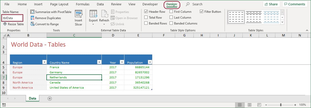
One of the first things that you should do when you create a table, is give it a name. It is not necessary, but if you don’t, Excel will do it for you. In that case, Excel will create a name like Table1, Table2 and so on. This obviously is not very helpful, as you never know what table it refers to.
You can change the default table name as follows:
-
- Select any cell inside the table
- Click the Design tab from the Table Tools
- Choose Properties > Table Name
I suggest that you always start the table name with the tbl abbreviation. This is a clear indication that you are referring to a table.
The table features are divided into five groups with specific functionality. Although this is nice, the most important features are not on the Design tab, but in the table itself!
1.3) Tables - Extra features
When you create a table:
-
- You can place an autofilter with sorting functionality on the header row
- You can display a Total Row, which has some powerful properties
- Added formulas refer to named (column) ranges and are easier to understand
Data selection is easier, because:
-
- When you move the cursor over the top left corner of the table, it becomes an arrow. You can now click to select all data and click again to select the header row as well
- When you move the cursor over a field header, it becomes an arrow. You can now click to select the data and click again, to select the field header as well
- When you move the cursor over the left column of a record, it becomes an arrow. You can now click to select the record
When you add a record to a table, by simply typing a new entry beneath the last record:
-
- Existing formatting is added
- Existing formulas are added
- Existing data validation is added

1.4) Tables - Functions
One of the features that make a table special, is the fact that functions and formulas are easier to maintain and better to understand. Take a closer look at Figure 1‑5. When you look at the Design tab from the Table Tools, you can see that the option to display a Total Row is not selected. When you check this box, the table adds a row that displays a sum (by default) for all columns.
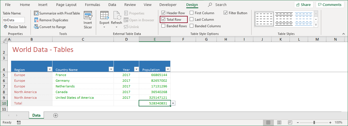
Although this is not extremely difficult, the solution is smart. When you select the total value for Population and press F2, the real SUM function appears.
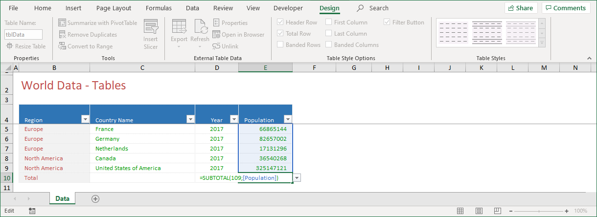
Figure 1‑7 shows that, instead of the SUM function, Excel uses the SUBTOTAL function to calculate the sum. Additionally, it shows that instead of a reference to a range, the table refers to the name of the column, or better, the name of the field. This makes error tracing and problem solving a lot easier.
But there is more. Did you ever try to use the SUM function to total a column of data in which some of the rows were hidden? If so, you probably got an unpleasant surprise. The SUM function calculates the total of all cells in that range, whether they’re visible or not. This means that the result won’t be the total of the numbers in the visible cells and that can be a problem. The way to avoid this, is to use the SUBTOTAL function and that is exactly what Excel does when you use its Total Row feature in a table.
This is valuable knowledge that you can instantly use. Consider this example. When you filter data, for instance, by Region, the Total row updates the total(s) and displays the result for that region. The numbers in the hidden cells won’t be added to this result. This is something that the SUM function won’t do and therefore is a very useful feature. The result of using the SUBTOTAL function is displayed in Figure 1‑8.
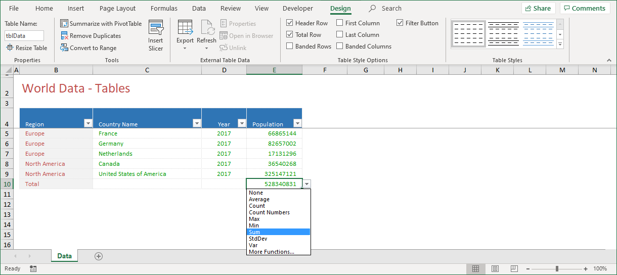
Also, notice the dropdown arrow next to the result in the Total row. When you click the arrow, you will find more options that you can use with the SUBTOTAL function. In total, the SUBTOTAL function has 11 functions that you can use to calculate results. This is very useful, but how does it work?
1.5) The SUBTOTAL function
The SUBTOTAL function uses other functions for subtotaling. In addition, it can include or exclude values in cells which are not visible. The SUBTOTAL function is designed for columns of data or vertical ranges. It is not designed for rows of data, or horizontal ranges. If there are subtotals within the used range, these nested subtotals are ignored to avoid double counting.
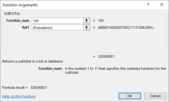
You can find the SUBTOTAL function in the MATH & TRIGONOMETRY category in the function library. Select the tab Formulas > Function library > Math & Trig > SUBTOTAL. When you insert the SUBTOTAL function, the following dialog pops up:
SYNTAX
=SUBTOTAL(Function_num; ref1; [refN]; …)
The SUBTOTAL function contains the following arguments:
- Function_num (Required)
- The numbers 1-11 and 101-111 specify the function that you want to use
- 1-11 > manually hidden rows are included
- 101-111 > manually hidden rows are excluded
- Cells hidden by a filter are always excluded
- Ref1 (Required)
- The first range or reference for which you want a subtotal
- RefN (Optional (2 to 254))
- Additional ranges or references for which you want a subtotal
1.5.1) SUBTOTAL - List of function numbers
De SUBTOTAL function, can include one of the following functions:
| 1/101 | AVERAGE | 7/107 | STDEV | ||
| 2/102 | COUNT | 8/108 | STDEVP | ||
| 3/103 | COUNTA | 9/109 | SUM | ||
| 4/104 | MAX | 10/110 | VAR | ||
| 5/105 | MIN | 11/111 | VARP | ||
| 6/106 | PRODUCT |
The SUBTOTAL function can include or exclude values in cells which are not visible. This behavior is reflected by the function number that you choose. As you can see from the function’s arguments, there are two series of function numbers. The first series (1-11) includes manually hidden rows. The second series (101-111) excludes manually hidden rows.
- Don’t forget that cells hidden by a filter are always excluded!
- Also notable is the fact that the SUBTOTAL function does not include other subtotals in the count.
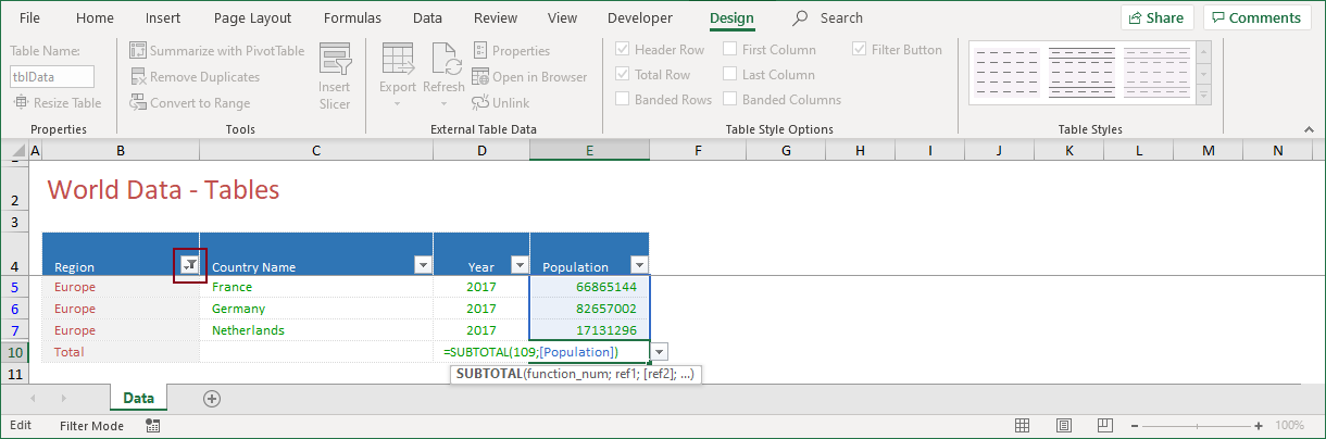
Figure 1‑10 shows a SUM for the Population field. The value 109 indicates that manually hidden rows are excluded from the count!
2) TABLES - FORMULAS
Another huge benefit of working with tables, is the readability and understandability of formulas. This can best be demonstrated with an example.
Let’s say that you want to calculate the country population in the table, when there is a 5% population growth. If you were working with a normal range, the formula you would enter in cell F5, would look like the one shown in Figure 2‑1. This formula would read =E5*105%.
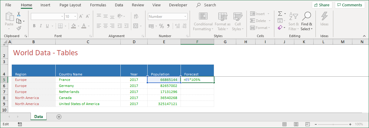
When you press Enter, the result is displayed in cell F5. You just need to copy the formula down to calculate the result for the other cells.
Although creating and copying formulas this way works fine, it has some pitfalls:
- A reference to a cell, does not ring a bell. When it comes to the readability of a formula, E5*105% does not mean much to most of us. Any alternative that explains the formula a bit more, is a better alternative.
- A possible error might occur when you create additional records. If you do so, you must not forget to copy the formula down. This is pretty simple, but is often forgotten!
2.1) Tables - Structured references
The issues that I described in §2 won’t occur when you convert a range into a table, as tables work with structured references. What does that mean?
When you create a table, Excel assigns a name to that table and to each column header in that table. Excel will also “save” those names in its internal memory. Of course, when you change the table name, that new name will overwrite the previous name.
When you add a formula to an Excel table by selecting cells within that table, the names appear automatically and replace the cell references. Here’s an example.
In Figure 2‑2, I entered the same formula by selecting cell E5 and typing *105%. While this range was converted to a table, Excel automatically displays the name of the field to which that cell reference belongs. In this case, Population.
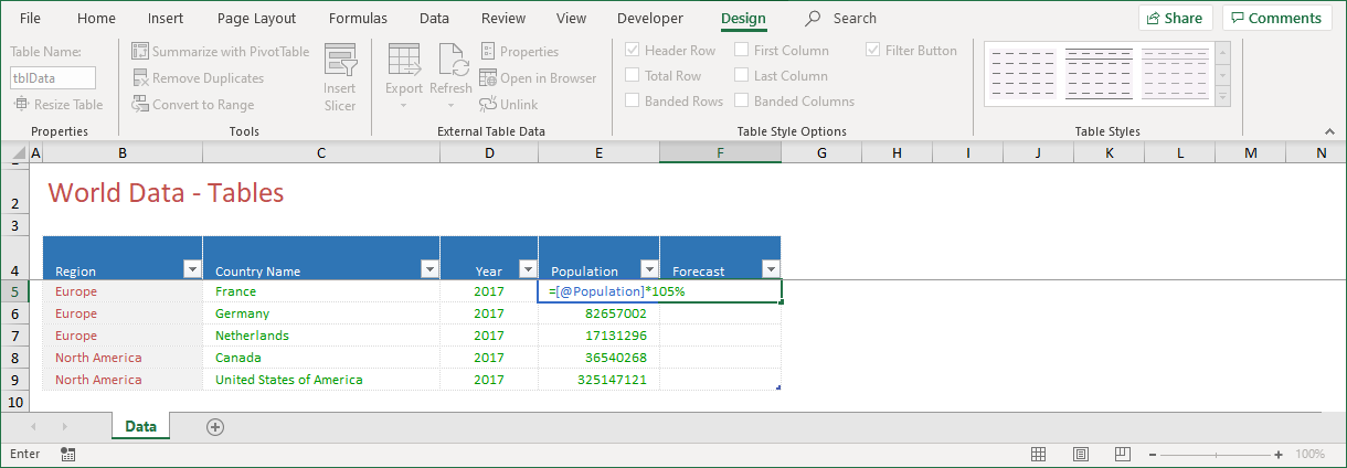
When I press Enter to complete my formula, the formula is automatically copied down to all the other cells in the table. This is an awesome extra feature that only a table offers. The formula that is now entered into all cells reads =[@Population]*105%. This is much more meaningful.
The use of brackets and the @ to refer to a table field, is called a structured reference, and the fact that tables work with structured references, gives you two valuable benefits. It makes formulas easier to understand and it minimizes the risk of errors. This is exactly what you want!
When you insert a formula outside of the table, the names or structured references also come into play.
In Figure 2‑3, the idea is to calculate the population of all the countries in the table. If I had not converted my range into a table, I would have had to include the whole range containing all countries in my formula. I would have had to type =SUM(E5:E9).
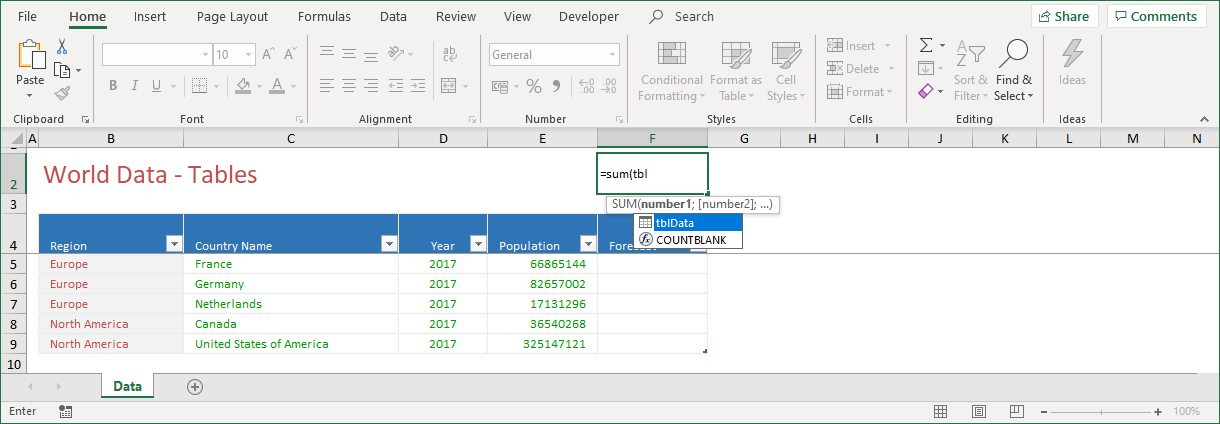
The fact that I did convert this range into a table, gives me the benefits of using the saved names and structured references in my formulas. In cell F2, I can now type the formula using the names which are stored in Excel’s memory. Another benefit of this method is that Excel automatically shows all available names that I can use.
When I type =SUM(tbl .. Excel immediately shows the name tblData. I just have to select that name an double-click it, to have Excel insert it into my formula. When I continue and type an open bracket sign ([), Excel shows the available options to add to my formula.
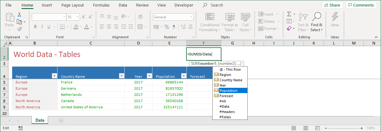
Again, I just have to select and double-click my choice, which is Population. When I add the close bracket character (]), I can press Enter and complete my formula.
- Be careful with formulas. You don’t have to type the formula close character to complete your formula, but you do have to insert the bracket characters to use the structured references.
Apart from this method, there is an even faster way of creating a formula outside of your table. In §1.3, I wrote that data selection is easier when you work with a table. In §1.5, I showed that the SUBTOTAL function offers some huge advantages over the normal SUM function. This is valuable knowledge.
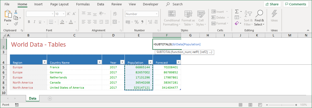
In Figure 2‑5, I inserted the SUBTOTAL function and chose the SUM option (9). I then moved my mouse pointer over the Population field name until it became an arrow. Excel now automatically extends my formula with tblData[Population], indicating that I want to SUM all the data from the Population field. When I press Enter, the result is there.
Now how cool is that!
3) TABLES - STYLES
When you create a table, you can add a style to it by selecting one from the Design tab on the ribbon. Excel has some 50 preformatted styles available to choose from, but in my opinion, none of them are very attractive. Luckily, you can create your own style.
In Figure 2‑5, I selected the table style Medium 2 but it isn’t visible. Is this a bug? Maybe, maybe not. The fact is that I formatted the range of cells before I converted it into the table. Apparently, this format remains active regardless of the style you choose!
3.1) Tables - Quick analysis
One of the new features in Excel, which is also available for a table, is the Quick Analysis Tool. The Quick Analysis Tool gives the option to analyze any selection of data in multiple ways. Figure 3‑2 shows that you can choose from Formatting, Charts, Totals, Tables and Sparklines. These features are not new and you might already know how they work, but the Quick Analysis Tool makes them easier to use and gives a better idea of available alternatives.

The crucial part in using the Quick Analysis Tool, is that you first have to select a range of data. This range must be a continuous range. After you selected a range of cells, the Quick Analysis icon appears at the bottom right of the selected data. When you click the icon, the tool itself becomes visible.
When the Quick Analysis tool is visible, you can select any of the features by clicking on it. When you then move the mouse pointer over the icons in the Quick Analysis tool, a preview of this selection is added to the table.
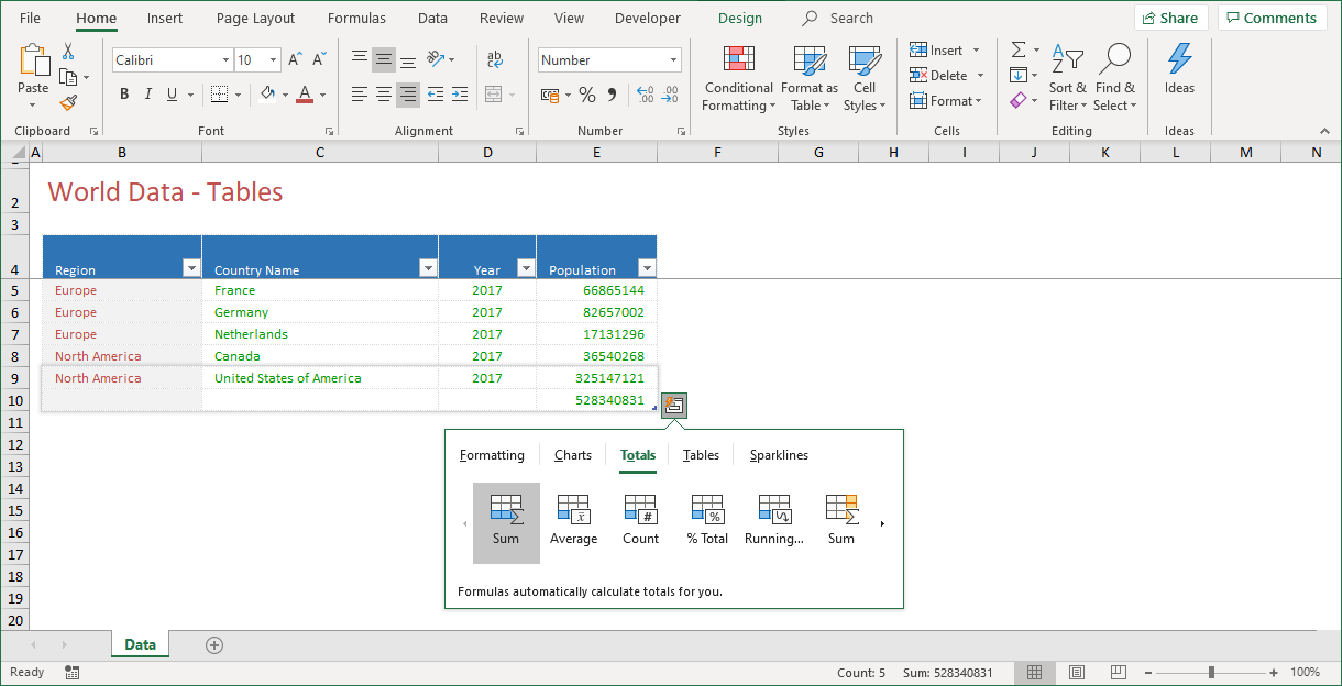
In Figure 3‑2, I selected the Sum function represented by the total of 528340831. If I had chosen Count, the result would have been 5.
!! Notice two different Sum icons on the Quick Analysis Tool. The left Sum icon resembles the rows, whereas the right Sum icon resembles the columns. You can also distinguish this difference from the bottom and right cell colors!
3.2) Tables - Dynamics
When you want to build a dashboard, there is another good reason to convert a range into a table: dynamics!
The core elements of a dashboard are pivot charts and pivot tables. These elements are both derived from a set of data. Mostly, this is a range. When you need to update a pivot chart or pivot table, you must also update the reference to that range, which takes a few mouse clicks.
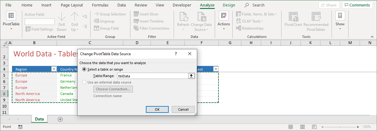
When you use a table as the data source for a pivot chart or a pivot table, you don’t need to update the reference to that range. The pivot table will refer to something like tblData, while tblData refers to a range, which is updated when a record is added or deleted. As you can see from Figure 3‑3, tblData refers to the entire range or data source!
This has two advantages. It saves a few mouse clicks and you can’t forget to update the reference to the data source. The one thing left is to refresh the pivot table and update the analysis. This is of course something that you should never forget!
But, as you will see in the article about pivot tables, a pivot table can be updated automatically, which saves us a few mouse clicks and minimizes the risk of errors!
4) SUMMARY
When you are building dashboards with Excel, it is essential that you work with a well-organized, structured set of data. A range, formatted as an Excel table, offers that structure and is a must have tool.
The dynamic features of a table make it a must-have tool when you are working with data. The key reason for using a table instead of a range, is the fact that it minimizes the risk of errors when you are processing data. Another good reason to use tables, is the fact that it makes formulas used in, or related to, the table easier to understand.
The SUBTOTAL function is just as useful as the table. The fact that this function uses or includes other functions and that it is able to exclude hidden data, makes it very versatile. In my opinion, the SUBTOTAL function is a function that you should also learn to master!
——————
This article is an extract from my book From Data 2 Dashboard in a Day. This book covers many more tools, tips and tricks about data that you use for dashboard reporting with Excel. You can purchase your copy here or see a preview in the book shop.